7 qPCR Analysis Technology Tips for Better Results?

Reliable qPCR results rarely come from pressing “run” and trusting the amplification plot. They begin with disciplined choices before the plate enters the instrument. Sample integrity, RNA purity, reverse-transcription consistency, primer design, and reference-gene stability can each change the final Cq value. Small errors become visible quickly.

Stephen A. Bustin, a leading authority on quantitative PCR and a contributor to the MIQE guidelines, has stressed that “qPCR is only as good as the quality of the data.” That principle shapes this guide. The seven qPCR analysis technology tips below connect practical laboratory habits with stronger analytical judgment. They cover calibration, replicate design, amplification efficiency, melt-curve interpretation, and transparent reporting. Each step matters.

Watch the controls.

A clean no-template control does not prove that every sample is reliable. It only reduces one concern. Likewise, a stable-looking amplification curve can hide inhibition or inconsistent pipetting. Experienced analysts inspect raw fluorescence, replicate spread, standard-curve behavior, and efficiency values together. They also question whether the chosen housekeeping gene remains stable under the tested treatment. That step is often skipped.

This overview is practical, but it is not a substitute for method validation. Instruments differ. Chemistries differ. Biological samples behave unpredictably. A protocol that works beautifully with purified DNA may fail with tissue-derived RNA. Careful analysts record those failures instead of quietly deleting inconvenient wells. Better qPCR analysis technology depends on reproducibility, clear documentation, and the willingness to challenge attractive results.

Table of Contents [Hide]

1 Define the qPCR Objective and Select an Appropriate Assay Design

2 Prepare High-Quality RNA, DNA Templates, and Reverse Transcription

3 Optimize Primers, Probes, and Reaction Conditions

4 Use Standards, Controls, and Replicates to Ensure Reliable Results

5 Validate Amplification and Analyze Cq Data Correctly

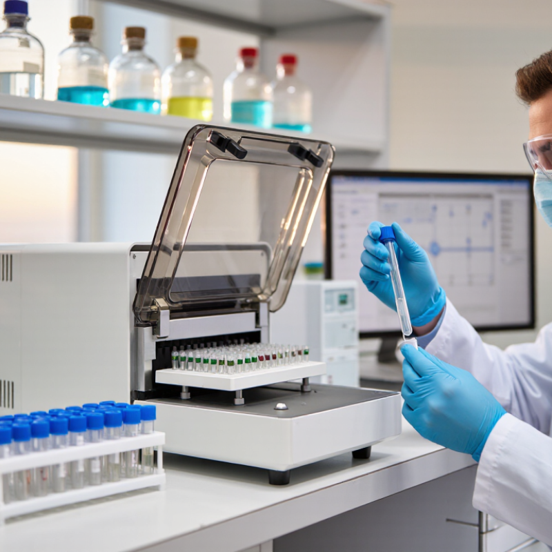
Define the qPCR Objective and Select an Appropriate Assay Design

A clear qPCR objective prevents expensive confusion. Decide whether you need absolute quantification, relative expression, genotyping, or detection. Each purpose demands a different assay design, control structure, and reporting threshold. “More data” is not always better data.

The MIQE guidance, published in Clinical Chemistry, reviewed 170 qPCR studies and highlighted frequent gaps in efficiency, specificity, and control reporting. That finding still matters. Before ordering primers, define the target transcript, expected abundance, sample type, and acceptable detection limit. For relative expression, verify stable reference genes under your exact treatment conditions. For absolute quantification, use a validated standard curve and report its efficiency, slope, and linear range. A practical efficiency range is commonly 90–110%. Outside it, pause and investigate.

Tips: Write the objective as one measurable sentence. Select amplicons across exon boundaries when genomic DNA may interfere. Keep the product short, ideally around 70–200 base pairs. Include no-template and reverse-transcription controls. Test specificity with melt-curve analysis or an independent method. The 2023 WHO laboratory quality-management guidance also stresses documented verification, traceability, and fit-for-purpose procedures. I sometimes overestimate a clean amplification curve. It can hide inhibition, poor normalization, or primer-dimer formation. Rechecking raw curves and sample history is worthwhile, even when the software reports success.

7 qPCR Analysis Technology Tips for Better Results? - Define the qPCR Objective and Select an Appropriate Assay Design

Tip	qPCR Objective	Recommended Assay Design	Key Data or Quality Checkpoint	Interpretation and Action
1	Define the measurement goal Determine whether the study requires relative expression, absolute quantity, pathogen detection, genotyping, or copy-number estimation.	Use comparative quantification for relative expression and a validated standard curve for absolute quantification. Select an endpoint that directly matches the biological question.	Predefine the target, sample groups, normalization strategy, and statistical comparison before running the assay.	A clear objective reduces unnecessary assay complexity and prevents inappropriate comparisons between relative and absolute results.
2	Choose the appropriate detection chemistry Balance specificity, multiplexing needs, assay development time, and cost.	Use a DNA-binding fluorescent dye for simple single-target assays with post-run melt-curve analysis. Use a sequence-specific probe when higher specificity, multiplexing, or discrimination of similar sequences is required.	Dye-based assays should show one specific melt-curve peak. Probe assays should include target-specific controls and demonstrate clear signal separation.	Unexpected melt peaks or nonspecific signal indicate that primer redesign, reaction optimization, or probe verification may be necessary.
3	Design a short, specific amplicon Improve amplification efficiency and reduce the impact of partially degraded nucleic acid.	A commonly used starting range is approximately 70–200 base pairs. Avoid known sequence variants, repetitive regions, strong secondary structures, and substantial complementarity between primers.	Verify a single expected product by melt curve, gel analysis, sequencing, or another suitable confirmation method during assay validation.	Multiple products, primer-dimers, or poor amplification efficiency require redesign or reaction optimization.
4	Control genomic DNA contamination Ensure that measured signal represents RNA-derived complementary DNA when analyzing gene expression.	Whenever possible, place primers across an exon–exon junction or design them in separate exons. Include an appropriate DNase treatment and a no-reverse-transcription control.	The no-reverse-transcription control should show no target amplification or only a signal outside the predefined acceptance range.	Signal in the no-reverse-transcription control suggests genomic DNA carryover and can invalidate expression measurements.
5	Use biologically stable reference genes Normalize technical variation without masking true biological changes.	Validate reference-gene stability in the same tissue, treatment, developmental stage, and experimental conditions. Use more than one stable reference gene when feasible.	Reference-gene expression should remain stable across the sample groups being compared; stability should be assessed with an appropriate validation method.	Do not assume that a commonly used housekeeping gene is stable under every biological condition.
6	Validate amplification performance Confirm that target and reference assays produce reliable quantitative data.	Prepare a serial dilution standard curve covering the expected concentration range. Evaluate slope, amplification efficiency, linearity, and reproducibility.	A commonly accepted starting criterion is approximately 90–110% amplification efficiency, corresponding to a slope near −3.58 to −3.10. An R² value of at least 0.98 is often used as a practical linearity benchmark.	Poor efficiency, curvature, or inconsistent replicate values may indicate inhibitors, pipetting error, poor primer design, or an unsuitable concentration range.
7	Build controls and replication into the design Distinguish true biological differences from contamination, background signal, and random measurement error.	Include no-template controls, positive controls where appropriate, biological replicates, and predefined technical replicates. Randomize sample placement when practical.	No-template controls should remain negative. Technical replicates should be assessed for consistency, and biological replicates—not technical replicates—should support biological inference.	Investigate outliers and control failures before averaging or applying statistical analysis; do not remove data solely to improve group separation.

Practical note: Acceptance criteria should be finalized during assay validation and applied consistently across the study. Efficiency and linearity targets may require adjustment when the sample type, chemistry, or quantification model differs.

Prepare High-Quality RNA, DNA Templates, and Reverse Transcription

7 qPCR Analysis Technology Tips for Better Results?

Reliable qPCR begins before the reaction. Use fresh, uncontaminated samples and record collection, storage, and thawing conditions. RNA should remain cold, because repeated freeze–thaw cycles can fragment transcripts. Check RNA integrity, not only concentration. A clear solution may still contain degraded RNA. For many workflows, an RNA A260/280 ratio near 2.0 is acceptable, while A260/230 values near 2.0 suggest fewer chemical contaminants. These ranges are commonly discussed in RNA quality guidance from Fleige and Pfaffl’s 2006 review. I still treat ratios as evidence, not proof.

Remove genomic DNA when measuring transcript abundance. Include a no-reverse-transcription control to expose DNA carryover. For DNA templates, quantify accurately and dilute concentrated extracts before amplification. Excess salts, phenol, or ethanol can inhibit polymerase activity. The MIQE guidelines recommend reporting template quality, input amounts, primer information, controls, and amplification efficiency. They identify 90–110% efficiency as a practical target, with a standard-curve slope close to −3.32 (Bustin et al., Clinical Chemistry, 2009).

Reverse transcription deserves equal attention. Keep RNA input consistent across samples, and use the same reaction conditions throughout the study. Random primers and oligo-based primers can produce different transcript coverage. Test the choice with your target biology. Include a reverse-transcription replicate when sample quantity allows. Small handling errors matter. My own weak point is assuming a successful cDNA yield means successful representation. It does not. Incomplete reverse transcription can quietly distort low-abundance targets and create confident-looking, misleading Ct differences.

Optimize Primers, Probes, and Reaction Conditions

7 qPCR Analysis Technology Tips for Better Results?
Optimize Primers, Probes, and Reaction Conditions

Primer design sets the ceiling for qPCR quality. Choose an amplicon between 70 and 200 base pairs. Keep primer lengths near 18–24 nucleotides. Their melting temperatures should differ by no more than 2°C. Check hairpins, self-dimers, and cross-dimers before ordering. Small mismatches matter. Avoid placing primers across highly variable regions or repeated sequences. A clean single product is more valuable than a high fluorescence signal.

Design the probe with a melting temperature about 5–10°C above the primers. Keep it away from strong secondary structures and avoid a guanine near the reporter end when possible. Test several concentrations rather than assuming the highest amount works best. In practice, excessive probe or primer can increase background noise. I have found that a modest concentration change sometimes improves the baseline more than a new instrument setting.

Reaction conditions deserve equal attention. Use consistent template volumes and mix gently without creating bubbles. Optimize the annealing temperature with a small gradient. Check magnesium concentration when amplification appears weak or nonspecific. Include no-template controls and, when relevant, a reverse-transcription control. A standard curve can reveal poor efficiency, but its correlation value alone is not enough. Aim for roughly 90–110% efficiency, then inspect the amplification plots manually. I still recheck dilution accuracy, because small pipetting errors can distort an otherwise promising assay.

Use Standards, Controls, and Replicates to Ensure Reliable Results

Reliable qPCR begins before the first sample enters the tube. Prepare a fresh standard series across the expected concentration range. Use at least five points, and inspect amplification efficiency rather than accepting a perfect-looking line. A strong curve can still hide pipetting errors. Include a no-template control in every run. It should remain quiet. If signal appears, investigate contamination, primer artifacts, or misplaced wells.

Controls need to answer specific questions. A positive control confirms that the reaction can detect its target. An extraction control reveals losses during sample preparation. For reverse-transcription assays, a minus-enzyme control helps identify genomic DNA carryover. Keep control materials separate from amplified products. Small habits matter. Use filtered tips, change gloves after setup, and record reagent lots and freeze-thaw history. These details make troubleshooting evidence-based instead of guesswork.

Run technical replicates, preferably three wells per sample when volume allows. Replicates expose uneven mixing and occasional pipetting mistakes. They do not repair poor sample quality. I once treated a single clean-looking well as reliable data; repeating the run changed the interpretation. That result was inconvenient, but useful. Set a predefined rule for acceptable replicate variation, then document exceptions instead of deleting awkward values. Review raw curves, not only reported quantification values. A late, irregular curve deserves attention, even when software assigns a number.

7 qPCR Analysis Technology Tips for Better Results

Use Standards, Controls, and Replicates to Ensure Reliable Results

This example uses a four-point, ten-fold standard series tested in triplicate. The mean Cq increases consistently as template concentration decreases, producing a standard-curve slope of approximately −3.33 cycles per log₁₀ dilution and an estimated amplification efficiency of about 100%.

Replicate Cq standard deviations ranged from 0.08 to 0.24 cycles. The no-template control remained undetermined, while the positive control produced a Cq of 25.6, supporting run validity and helping distinguish true amplification from contamination or inhibition.

Validate Amplification and Analyze Cq Data Correctly

qPCR Analysis Technology Tips for Better Results?

Validate Amplification and Analyze Cq Data Correctly

Reliable qPCR begins with validated amplification, not attractive fluorescence curves. Check primer specificity with melt-curve analysis or gel electrophoresis when appropriate. A single sharp melt peak supports specificity, but it does not prove perfect efficiency. Run a standard curve across several template concentrations. Record its slope, efficiency, and linearity. Efficiencies near 90–110% are commonly acceptable, although assay design and sample type can shift results. Include no-template controls in every run. A signal there may indicate contamination or primer-dimer formation. Repeat suspicious wells rather than quietly deleting them. Small details matter.

Keep reaction volumes, template input, and cycling conditions consistent. Use technical replicates, preferably three wells, to identify pipetting variation. Examine replicate Cq values before calculating averages. A large spread deserves investigation. Do not compare raw Cq values from different assays without normalization. Select stable reference genes and verify their stability across the tested samples. Analyze relative expression with a validated comparative-Cq approach only when amplification efficiencies are sufficiently similar. Otherwise, use efficiency-corrected calculations.

Low Cq means more starting template, not automatically higher biological expression. Check whether the baseline, threshold, and fluorescence traces are reasonable. Avoid moving the threshold simply to improve agreement. That is tempting, but scientifically weak. I have seen clean-looking data change after one poorly mixed dilution was removed. The lesson is uncomfortable: technical judgment can introduce bias. Keep an audit trail, inspect outliers, and report exclusions with clear reasons. Cq values are measurements, not conclusions.